Identify and Plot the TID Maxima and Minima

This example recreates Figure 13 from the manuscript this repository supports. It uses the model run loaded in Download Model Data.

import datetime as dt
import numpy as np
import lstid_processing.model as lsmod

# Define the plot time range
estart = dt.datetime(2014, 3, 25, 22)
estop = dt.datetime(2014, 3, 26, 6)

nt_start = lsmod.analysis.get_time_index(sami['datetime'].values, estart)
nt_stop = lsmod.analysis.get_time_index(sami['datetime'].values, estop) + 1

# Get the field-line indices
(nlind, nfindc, nfindd, nt, nzindc,
 nzindd) = lsmod.analysis.get_default_indices(sami['datetime'].values,
                                              sami['glat'].values)

# Find the F2 peak locations for this period
f2_inds = lsmod.analysis.get_f2_peaks(nlind, nfindd, sami)

# Define the topside as the altitude range between the highest F2 peaks
nzinds = np.arange(f2_inds['south'][nt_start:nt_stop].min(),
                   f2_inds['north'][nt_start:nt_stop].max() + 1, 1)

# Create the plot and get the analysis data
out = lsmod.plots.get_plot_tid_peaks(sami, nt_start, nt_stop, nlind, nfindd,
                                     nzinds, 'd', add_lines=True)

# Get the figure handle and add a figure title
fig = out[-1]
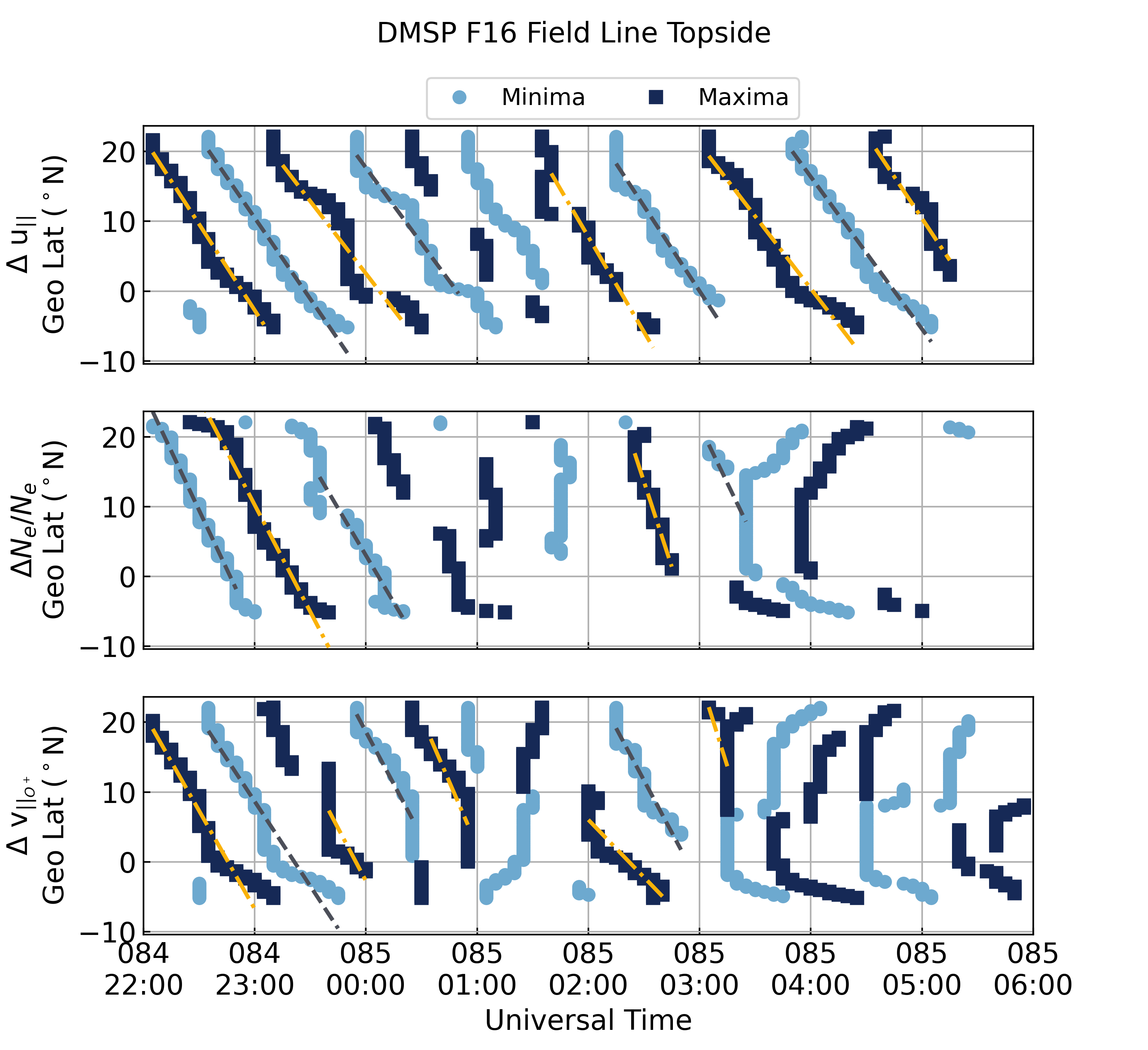
fig.suptitle('DMSP F16 Field Line Topside', fontsize='medium')

This will create the figure below.